Performance Analysis of Long Flow Lines with Finite Buffer Sizes by Decomposition
Flow lines comprising only two or three stations can be evaluated with exact methods under certain conditions. However, for larger flow lines this option is not available. For these systems there are several approximation methods available, which use the so-called "decomposition approach".
If the buffers sizes are not finite, then the performance of the complete flow production system can be deducted from the performance of the bottleneck of the system. The bottleneck can be easily identified by looking at the isolated efficiencies of the stations (or the processing rates). However, with finite buffers, the productivity of a station can be degraded by blocking. If breakdowns are possible, a station can be down. Hence, we must consider four states of a station: busy, idle, blocked, down.
Let us show how the decomposition approach is used for the analysis of a linear flow production system. Consider a system with the following characteristics:
- Asynchronous material flow
- Exponential-distributed processing times
- No breakdowns
- Finite buffer sizes
- The first station is never starved
- The last station is never blocked
The assumptions of exponential-distributed processing times and no breakdowns are rarely met in industrial practice. However, for industrial applications there are modified procedures available, which have successfully been applied in many companies. For more information, see POM Flowline Optimizer.
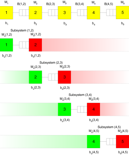
Consider a flow line consisting of M=5 stations as shown by the yellow squares in the following figure.

This system is decomposed into (M-1)=4 subsystems consisting of two stations each. Each of the two-station subsystems is analysed with the help of an exact or approximate evaluation method. The parameters of the two stations of the subsystem are then adjusted such that they account for the effects of all stations located outside the subsystem. All results are then adjusted in an iterative procedure.
In the above figure, for the easy identification of the subsystems the original numbers of the stations are shown in brackets. $b_m$ is the mean processing time of station $m$ (later we will calculate with the processing rate $\mu_m=\frac{1}{b_m}$). $M_u$ is the upstream-station of a system. $M_d$ is the associated downstream-station. $b_u(m,m+1)$ is the modified processing time of the upstream-station of the subsystem consisting of stations $m$ and $m+1$. $b_d(m,m+1)$ is the modified processing time of the downstream-station of the subsystem consisting of the stations $m$ and $m+1$.
Each subsystem (comprising the original stations $m$ and $m+1$) has a upstream-station $M_u(m,m+1)$ (which is never starved) and a downstream-station $M_d(m,m+1)$ (which is never blocked). These stations are separated by a buffer with capacity $c_{m,m+1}$. Consider the buffer between the stations 2 and 3:
 Now, assume there is someone monitoring the inflow of workpieces into this buffer.
  The observer only sees the inflow of workpieces into the buffer. The arrival rate of workpieces into the buffer depends on the upstream station, particularly on its processing rate and on the fact whether the upstream is not starving.
In the two-station model, by assumption the first station is never starved. However, in reality, the upstream station may be starved, because its upstream station (in the real system station 1) may sometimes work too slow. As the observer does not see station 1, we must find a way to account for the starving effects in the characterisation of the inflow into the buffer.  Now, let's monitor the outflow of workpieces out of the buffer:
 The outflow depends on the processing speed of the downstream station and on the fact whether the downstream station is not blocked.
 In the two-station model, by assumption the second station is never blocked. In reality, however, the downstream station may be blocked, because its downstream station (in the real system station 4) sometimes may work too slow. As the observer does not see station 4 either, we must find a way to account for the blocking effects in the characterisation of the outflow from the buffer.
 The observer can only see the direct inflow into and the direct outflow from the buffer. He does not see the reason why the inflow or outflow are sometimes slow (or may blocked by its own downstream station), and, consequently, can only estimate the amount of starving and blocking of the stations 2 and 3, respectively. This estimation can be accomplished as follows. Let
- $\mu_u =\frac {1}{b_u}$ be the adjusted processing rate of the upstream-station (including the effects of starving)
- $\mu_d = \frac {1}{b_d}$ be the adjusted processing rate of the downstream-station (including the effects of blocking)
The rate $\mu_u$ accounts for all effects resulting from processing and starving of all stations located upstream from the buffer. The rate $\mu_d$ accounts for all effects resulting from processing and blocking of all stations located downstream of the buffer.
Let us assume, that the adjusted processing rates $\mu_d(m,m+1)$ of all downstream-stations are known. These $\mu_d$-values do not contain the starving-effects, but the blocking-effects. If these are estimated correctly, then everything is fine, otherwise, we will have to update them. For the moment we assume them as given. At the beginning, plausible starting values could be $\mu_d(m,m+1)=\mu_{m+1}$ ($m+1=2,\ldots,M$). Obviously, this is a very optimistic estimation of the system performance, as the influence of blocking will result a loss of throughput.
Calculation of the $\mu_u-$values:
The $\mu_u$-values are the processing rates of the upstream-stations. They include the starving-effects of all stations located upstream of a focussed two-station-subsystem.
As the first station of the flow production system (station 1) is never starved, we set
$\frac{1}{\mu _u\left( {1,2} \right)}=\frac{1} {\mu _1}$
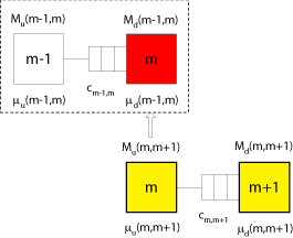
For all other stations $(2,3,\ldots,M)$ we consider the following figure:
Assume that we have analysed subsystem ($m-1,m$) already, and that we know the rate $\mu _u\left( {m-1,m} \right)$. As noted earlier, $\mu _d\left( {m-1,m} \right)$ is assumed to be known as well. In this case, the exact throughput of the subsystem $(m-1,m)$, $X(m-1,m)$ can be calculated with an appropriate model such as a Markov model. The calculation of the throughput of a two-station-subsystem is shown in detail here (in german) and can be found in any textbook on stochastic models of manufacturing systems.
The processing rate $\mu _u(m,m+1)$ of the upstream-station of subsystem $(m,m+1)$ accounts for the processing time plus the additional starving time, which is currently unknown. Unfortunately, by assumption the upstream-station in a subsystem is never starved. However, we note that the stations $M_u(m,m+1)$ and $M_d(m-1,m)$ are the identical, as they both stand for station $m$ of the original system.
So, assume the throughput of subsystem $(m-1,m)$, $X(m-1,m)$ is known. This throughput must be less than the isolated processing rate $\mu_m$ of station $m$, as it includes the effects of starving and blocking in the of subsystem $(m-1,m)$. From $X(m-1,m)$ we obtain the average inter-departure time of workpieces as $\frac{1}{X(m-1,m)}$. If the downstream-station were never starved, it could work with the processing rate $\mu_d(m-1,m)$ (which is greater than $X(m-1,m)$) and the average inter-departure time of subsystem $(m-1,m)$ were $\frac{1}{\mu_d(m-1,m)}$. Now, if the downstream-station of subsystem $(m-1,m)$ can work faster than the subsystem $(m-1,m)$, than it will be starved once and again. Hence, the average starving time is the difference of $\frac{1}{\mu_m}$ and $\frac{1}{X(m-1,m)}$. Thus, we can derive $\mu_u(m,m+1)$ from $X(m-1,m)$ and $\mu_d(m-1,m)$ as follows:
$\frac{1}{\mu _u\left( {m,m+1} \right)} =\frac{1}{\mu _m}+ \underbrace{\left[ {\frac{1}{X\left( {m-1,m} \right)}- \frac{1}{\mu _d\left( {m-1,m} \right)}} \right]}_{\mathrm{= average starving time}} \qquad m=2,3,...,m-1 $
The calculation of the throughput $X(m-1,m)$ is implemented in the Production Management Trainer.
Calculation of the $\mu_d-$values:
The $\mu_d$-values are the processing rates of the downstream-stations. They include the blocking effects resulting from all stations located downstream of a focussed two-station- subsystem.
As the last station of the system is never blocked, we set
$\frac{1}{\mu _d\left( {M-1,M} \right)}=\frac{1} {\mu _M}$
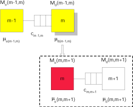
For all other stations we consider the following figure:

The remaining argumentation is similar to that used in the calculation of the starving times.
The processing rate $\mu_d(m-1,m)$ of the downstream-station of subsystem $(m-1,m)$ accounts for the processing time plus the additional blocking time, which is currently unknown. Unfortunately, by assumption the downstream-station in a subsystem is never blocked. However, we observe that the stations $M_d(m-1,m)$ und $M_u(m,m+1)$ are identical, as they both stand for station $m$ of the original system.
Assume now, that the throughput of subsystem $(m,m+1)$, $X(m,m+1)$, is known. Assume also, that the adjusted processing rate of the upstream-station $M_u(m,m+1)$, $\mu _u\left( {m,m+1} \right)}$, has been calculated (this has been shown above). Then the average blocking time of the upstream-station $M_u(m,m+1)$ can be calculated from the throughput of the subsystem and the adjusted processing rate of the upstream-station $M_u(m,m+1)$ as follows:
$\frac{1}{\mu _d\left( {m-1,m} \right)} =\frac{1}{\mu _m}+ \underbrace{\left[ {\frac{1}{X\left( {m,m+1} \right)}- \frac{1}{\mu _u\left( {m,m+1} \right)}} \right]}_{\mathrm{average blocking time}} \qquad m=M-1,M-2,...,2$
The solution of this set of equations goes as follows: Start with assuming the downstream processing rates as given and calculate the upstream processing rates $(2,3,\ldots,M)$. Then recalculate the downstream processing rates $m=M-1,M-2,...,2$. Repeat these steps until the throughputs of all subsystems are (almost) equal and a stable solution has been found.
The complete decomposition approach is implemented with an option to show each detailed calculation step in the Production Management Trainer.
For industrial applications (based on different assumption concerning the processing times and the possible occurrence of breakdowns), the software system POM Flowline Optimizer basically uses this type of decomposition to analyse and optimise flow lines with limited buffers among the stations. For many years, it has been successfully applied in industrial companies for the optimization of automobile body shops or for the the design of flow lines in the electronics industry.